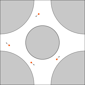
Standard table, obstacles are two disks:
at (0, 0) of radius 0.4 and
at (0.5, 0.5) of radius 0.2
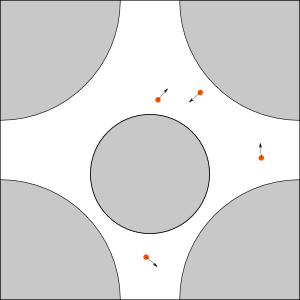
A little bit modified standard table: position of smaller obstacle is (0.5, 0.42)
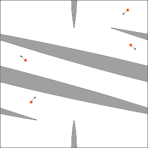
Simple table made to be different from standard table. Consists of four arcs of a circles.
Mean free paths:
- "discrete": 0.31
- "continuous": 0.245
Conductivity matrices:
- 1 particle: $$ \left( \begin{matrix} 0.0893 & -0.0007 \\ -0.0007 & 0.0892 \end{matrix} \right) $$
- 5 particles: $$ \left( \begin{matrix} 0.136 & -7.62 \times 10^{-5} \\ -7.62 \times 10^{-5} & 0.136 \end{matrix} \right) $$
- 10 particles: $$ \left( \begin{matrix} 0.139 & -0.0001 \\ -0.0001 & 0.139 \end{matrix} \right) $$
Mean free paths:
- "discrete": 0.31
- "continuous": 0.25
Conductivity matrices:
- 1 particle: $$ \left( \begin{matrix} 0.0978 & 9.97 \times 10^{-5} \\ 9.97 \times 10^{-5} & 0.0692 \end{matrix} \right) $$
- 5 particles: $$ \left( \begin{matrix} 0.146 & -3.09 \times 10^{-5} \\ -3.09 \times 10^{-5} & 0.104 \end{matrix} \right) $$
- 10 particles: $$ \left( \begin{matrix} 0.152 & 0.0002 \\ 0.0002 & 0.107 \end{matrix} \right) $$
Mean free paths:
- "discrete": 0.431
- "continuous": 0.357
Conductivity matrices:
- 1 particle: $$ \left( \begin{matrix} 0.461 & -0.159 \\ -0.159 & 0.0783 \end{matrix} \right) $$ e-values: 0.0209 and 0.518
- 5 particles: $$ \left( \begin{matrix} 0.705 & -0.242 \\ -0.242 & 0.12 \end{matrix} \right) $$ e-values: 0.033 and 0.792
- 10 particles: $$ \left( \begin{matrix} 0.718 & -0.25 \\ -0.25 & 0.124 \end{matrix} \right) $$ e-values: 0.0327 and 0.809